Analysis of Covariance is an analytical technique that combines elements of ANOVA and regression theory. This is best illustrated by an example. Consider the data set below. The research question we want to answer is: Do different types of fertilizers have different effects on the final height of tomato plants? The dependent (response) variable is the final height of tomato plants at 10 weeks. The factor of interest is the type of fertilizer used after transplanting. Three varieties of fertilizers were used.  Since there was a variation in the initial heights of plants at the time of transplantation, the initial value is entered as covariate in order to determine whether the type of fertilizer makes a difference in the final height of tomato plants after 10 weeks while controlling for the initial height.

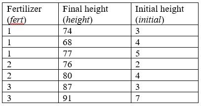
ANCOVA Table 1

Testing Assumptions: Homogeneity of Regression Slopes

Before we can start the analysis, we need to check the assumption that the regression of final height on initial height is the same for all three types of fertilizer. This is known as assumption of equality (homogeneity) of regression slopes. This can be tested by fitting a model containing main effects of fert and initial, as well as the fert*initial interaction. The interaction term provides the test of the null hypothesis of equal slopes.

Using the information on Table 1 above create an SPSS data file. To produce the output, after creating the data file, from the menus choose:

Analyze

            General Linear Model

                        Univariate…

Dependent Variable: height

Fixed Factor(s): fert

Covariate(s): initial

Model…

            Select Custom

            Model: fert initail fert*initial  

Click on Continue

Options…

Display

            Select Observed power

Click on Continue and then OK

Examine the output table Test of Between-Subjects Effects and try to interpret it. Does the interaction term fert*initial show any evidence of violation of the equal slopes assumption?

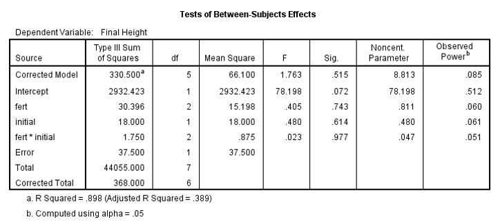
ANCOVA Table 2

The interaction term fert*initial shows no evidence of violation of the equal slopes assumptions. The F value is 0.023 with a p-value of 0.977. We can proceed to estimate the effects of fertilizer type on final height given the initial height.

Now, we can proceed with the analysis knowing that the slopes are equal for different type of fertilizers. However, is there anything else that you should worry about the data?

Yes, the small sample size of the data set. However, the data is use to illustrate the steps involved in this type of analysis.

Analysis-of-Covariance Model (ANCOVA)

To produce the analysis-of-covariance results, recall the GLM Univariate dialogue box, or from the menus choose:

Analyze

            General Linear Model

                        Univariate…

Dependent Variable: height

Fixed Factor(s): fert

Covariate(s): initial

Model…

            Select Full factorial

Click on Continue

Options…

            Estimated Marginal Means

            Display means for: fert

Display

            Select Parameter estimates

            Select Observed power

Click on Continue and then OK

Examine and attempt to interpret the output.

Looking at the Tests of between-subjects effects table shown below, there is some evidence of a fertilizer effect: the F value is 9.294 with a p-value of 0.052.

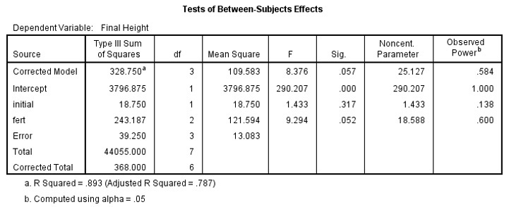
ANCOVA Table 3

From the Parameter estimate table shown below, we can write the following equation:

Mean Final Height = 82.750 – 14.750 x fert1 – 8.5 x fert2 + 4x1.25            …… equation 1

The coefficient 4 is the average of initial height of the tomato plants.

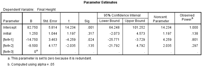
 ANCOVA Table 4

Fertilizer 3 (Fert=3) is the reference category. We can use equation 1 to calculate the Estimated marginal means as shown on the table.

Attempt these calculations.

Fertilizer 1: 82.750 – 14.750 x 1 – 8.5 x 0 + 4x1.25 = 73                  (here fert2=0)

Fertilizer 2: 82.750 – 14.750 x 0 – 8.5 x 1 + 4x1.25 = 79.25             (here fert1=0)

Fertilizer 3: 82.750 – 14.750 x 0 – 8.5 x 0 + 4x1.25 = 87.75             (here fert1= and fert2=0)

Estimated Marginal Means

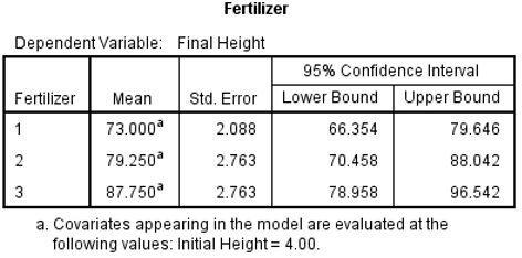
ANCOVA Table 5

Summary

By specifying an interaction between the covariate (initial height) and factor (fertilizer), you were able to test the homogeneity of the covariate parameter estimates across levels of fertilizer. Since the interaction term was not significant (p=0.977), indicating the covariate parameter estimates are homogenous, you proceeded with an analysis of covariance and found that fertilizer has an effect. That is, the final height of tomato plant using fertilizer 1 is 14.75 lower than tomato plant using fertilizer 3 (p=0.024).  The final height of tomato plant using fertilizer 2 is 8.5 lower than plant using fertilizer 3 but not significantly different (p=0.135).   

What if the Assumption is violated?

If your data failed the homogeneity of regression slopes, you could estimate a model incorporating separate slopes.

To obtain these separate slope estimates, recall the GLM Univariate dialogue box, or from the menus choose:

Analyze

            General Linear Model

                        Univariate…

Dependent Variable: height

Fixed Factor(s): fert

Covariate(s): initial

Model…

            Select Custom

            Model: fert fert*initial (initial is removed)

            Deselect Include intercept in the model

Click on Continue

Options…

            Parameter estimates

            Observed power

Click on Continue and then OK

Examine the output.

Look at the Parameter Estimates table.

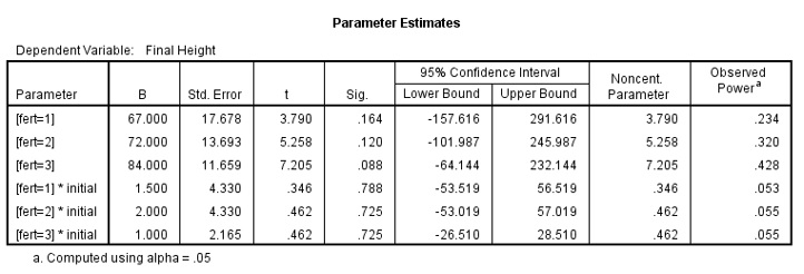
ANCOVA Table 6

For each level of fertilizer the prediction equations are:

Fertilizer =1: Final Height = 67 + 1.5 x initial

Fertilizer =2: Final Height = 72 + 2 x initial

Fertilizer =3: Final Height = 84 + 1 x initial