‌‌‌‌‌ 

Life Tables: Use life tables if cases can be classified into meaningful equal time interval. Life table can be used to calculate the probability of a terminal event during any interval under study.

Kaplan-Meier: Use this technique if cases cannot be classified into equal time intervals as above. This is common to many clinical and experimental studies.

Cox Regression: Use this technique if you want to see the relation between survival time and a predictor variable, for instant age or tumour type.

Kaplan-Meier Survival Analysis Example

A pharmaceutical company is developing an anti-inflammatory medication for treating chronic arthritic pain. Of particular interest is the time it takes for the drug to take effect and how it compares to an existing medication. Shorter times to effect are considered better.

The results of a clinical trial are collected in pain_medication.sav, which is stored in this folder \\campus\software\dept\spss. Open the file and study it. Note that the trial have 200 patients, 104 on new treatment and 96 on existing treatment. Use Kaplan-Meier Survival Analysis to examine the distribution of "time to effect" and compare the effectiveness of the two treatments.

• To run a Kaplan-Meier Survival Analysis, from the menus choose:

Analyze
  Survival
    Kaplan-Meier...

• Select Time to effect [time] as the Time variable.

• Select Effect status [status] as the Status variable.

• Click Define Event.

• Under Value(s) Indicating Event Has Occurred type 1 in the text area next to Single value:.

• Click Continue.

• Select Treatment [treatment] as a Factor.

• Click Compare Factor.

• Select Log rank, Breslow, and Tarone-Ware.

• Click Continue.

• Click Options in the Kaplan-Meier dialog box.

• Select Quartilesin the Statistics group and Survival in the Plots group.

• Click Continue.

• Click OK in the Kaplan-Meier dialog box.

Interpretation

Case Processing Summary Table

The case processing summary table shown below provides some vital information about the treatment groups. Of the 200 patients who took part in the clinical trial 153 experience the terminal event and 47 were censored (did not experience the terminal event). Terminal event here is how quickly the patients were free of pain after taking the medication. Of the 104 patients on the new treatment, 79 experienced the terminal event and 25 did not. For the other group the corresponding numbers are 74 and 22 respectively.

Survival Figure 1

Survival Table

The survival table is a descriptive table that details the time until the drug takes effect. The table is sectioned by each level of Treatment, and each observation occupies its own row in the table. Normally, you will not include this table in your write up, but you can put it in an Appendix. The first five rows of the table for each group is shown below:

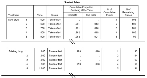
Survival Figure 2

Time: The time at which the event or censoring occurred.

Status: Indicates whether the case experienced the terminal event or was censored.

Cumulative Proportion Surviving at the Time: The proportion of cases surviving from the start of the table until this time. When multiple cases experience the terminal event at the same time, these estimates are printed once for that time period and apply to all the cases whose drug took effect at that time.

 N of Cumulative Events: The number of cases that have experienced the terminal event from the start of the table until this time.

N of Remaining Cases: The number of cases that, at this time, have yet to experience the terminal event or be censored.

Survival Functions (Curves)

The survival curves give a visual representation of the life tables. The horizontal axis shows the time to event. In this plot, drops in the survival curve occur whenever the medication takes effect in a patient. The vertical axis shows the probability of survival. Thus, any point on the survival curve shows the probability that a patient on a given treatment will not have experienced relief by that time.

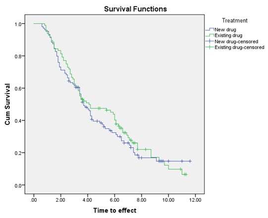
Survival Figure 3

The plot for the New drug below that of the Existing drug throughout most of the trial, which suggests that the new drug may give faster relief than the old. To determine whether these differences are due to chance, look at the comparisons tables.

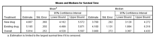
Mean and Medians for Survival Time

The means and medians for survival time table offers a quick numerical comparison of the "typical" times to effect for each of the medications. Since there is a lot of overlap in the confidence intervals, it is unlikely that there is much difference in the "average" survival time. On average, patients on the new treatment got quicker relief from pain compared to patients on the existing treatment (4.867 v 5.185).

 Survival Figure 4

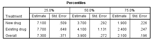
Percentiles

The percentiles table gives estimates of the first quartile, median, and third quartile of the survival distribution. The interpretation of percentiles for survival curves is that the 75th percentile is the latest time that at least 75 percent of the patients have yet to feel relief.

Survival Figure 5

Overall Comparisons

This table provides overall tests of the equality of survival times across groups. Since the significance values of the tests are all greater than 0.05, you cannot determine a difference between the survival curves. Log rank is the standard test, Breslow gives more weight to early cases and Tarone-Ware weights early cases somewhat less heavily.

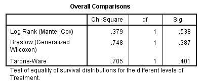
 Survival Figure 6

Summary

With the Kaplan-Meier Survival Analysis procedure, you have examined the distribution of time to effect for two different medications. The comparison tests show that there is not a statistically significant difference between them.