How to perform and interpret Binary Logistic Regression Model Using SPSS

Introduction

Binary logistic regression modelling can be used in many situations to answer research questions. You can use it to predict the presence or absence of a characteristic or outcome based on values of a set of predictor variables. You can use binary logistic regression to answer the following questions amongst others:

• What factors influence student retention / drop out on a particular course?
• What are the risk factors for heart disease?
• What factors influence customers to stay or leave a company?

Assumptions

• Logistic regression does not rely on distributional assumptions in the same sense that other procedures does. However, your solution may be more stable if your predictors have a multivariate normal distribution. Additionally, as with other forms of regression, multicollinearity among the predictors should be avoided. The dependent variable should be truly dichotomous (present / absent, event / no event, or yes / no), usually coded using 1=Yes and 0=No. Independent variables can be continuous or categorical; if categorical, they should be dummy or indicator coded (there is an option in the procedure to recode categorical variables automatically).
• Observations should be independent

Binary Logistic Model

In this type of model you estimate the probability of an event occurring. The model can be written as:

For a single independent variable

For many independent variables:

where b₀ and b₁, b₂, are coefficients estimated from the data, x₁, x₂, are the independent variables, n is the number of independent variables and e is the base of natural logarithms (2.781).

Example 

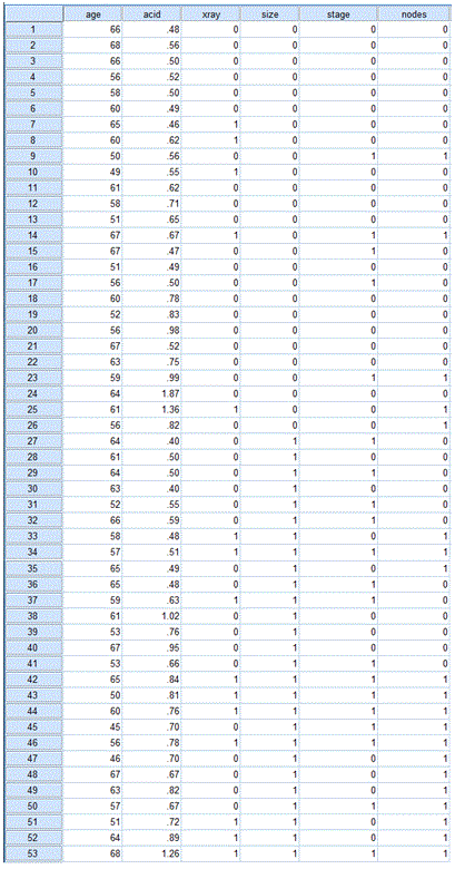
The data held in the file cancer.sav is from a study reported by Brown (1980) and are commonly cited in texts considering binary logistic regression. The prognosis for prostate cancer is based upon whether or not the cancer has spread to the surrounding lymph nodes. In this classic study Brown et al (see Brown, 1980) explored the following separate indicators for lymph node involvement in a group of 53 men known to have prostate cancer.

Preparing the Data set

Use the information on the table below to prepare the data file before you begin the analysis.

The variables (corresponding to columns in the data file) are:

          1) age - age of patients in years.
          2) acid - level of serum acid phosphates (acid level in King-Armstrong units)
          3) xray - x-ray result (0 = negative, 1 - positive)
          4) size - size of tumor (0 = small, 1 = large)
          5) stage - stage of tumor (0 = less serious, 1 = more serious)
          6) nodes - nodal involvement (0 = not involved, 1 = involved)

The data file is shown below:

Checking Assumptions

Binary logistic regression is most effective when the dependent variable is truly dichotomous not some continuous variable that has been categorized. It is clear that the dependent variable nodes is dichotomous with codes (0 = not involved, 1 = involved). Normality test indicates that of the two continuous variables age is just normally distributed (p=0.064) while acid is not (p=0.005); so in essence the data fails the multivariate normal distribution test. Some sort of transformation will be needed for acid. I recommend the Blom’s Normal Score transformation. In this example, I will not do any transformation, I will use the data as it was originally presented by Brown et al. (Brown, 1980). There is little correlation between age and acid (r=-0.12). The observations are independent of each other.

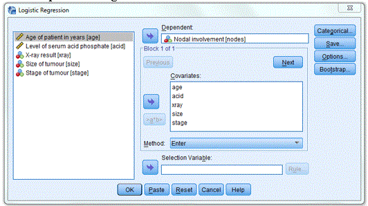
Running the Binary Logistic Regression Procedure

Analyze -> Regression -> Binary Logistic….

Dependent: Nodal involvement [nodes]

Covariates: age acid xray size stage (Note that you do not need to specify xray size and stage as categorical variables as they are coded as 1 and 0)

Save…: Under Predicted Values select Probabilities and Group membership

Options…: CI for exp(B)

Method: Enter (Note that you can select other method e.g. stepwise)

The completed dialogue box is shown below:

Interpretation of Output

The selections made above generate lots of output. The interpretation of the relevant output is discussed below.  The generated output is separated into two blocks Block 0 and Block 1.

Block 0: Beginning Block

At the beginning block none of the predictors are in the model equation, only the constant (  is present in the model.

Classification Table

The first relevant output from the beginning block is the classification table.

We see that the constant only model is doing a good job at predicting nodal involvement for not involved 100% correct but the model is doing a terrible job in predicting nodal involvement for involved 0% correct. The overall correct percentage prediction rate is 62.3%.

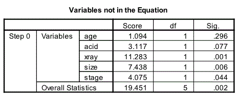
Variables not in the Equation Table

The next relevant output from the beginning block is the Variables not in the Equation table.

Here we see all the predictor variables that have not yet entered the model. This also the last output from Block 0.

Block1: Method=Enter

For Block1 the first relevant output is Omnibus Tests for Model Coefficients table. This table compares the constant only model to the model with all the predictors. The model with all the predictors is significantly better than the constant only model [Chi-Square=22.126, df=5 and p=0.001 (<0.05)].

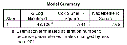
Model Summary

The next relevant output is the Model Summary table. This provides information about the goodness of fit of the model. Two measures are given Cox & Snell R Square and Nagelkerke R Square. Nagelkerke R Square is commonly used as the former does not scale up to 1. From Nagelkerke R Square it is clear that 46.5% of the variation in nodal involvement is account for by age acid x-ray size and stage.

Hosmer and Lemeshow test

This output tells you if the model fits the data. We can conclude that the model fits the data [Chi-Square=5.954, df=8 and p=0.652 (>0.05)].

Classification Table

The next relevant output is the Classification Table. This compares the model predictions to the actual observation. The model is doing a reasonable job in predicting men who do not have malignant node compared to those who do; i.e. 84.8% vs 65.0%. Overall 77.4% of the 53 men were correctly classified. It is possible to examine the probability of nodal involvement for each man; as this was requested during the analysis the probabilities will be saved as part of the data file.

Variable in the Equation

The next relevant output is the Variable in the Equation Table. This is one of the most useful outputs. It shows the estimated coefficients for age, acid, xray, size, stage and the constant under the column heading B. In order to interpret the coefficient it is advisable to convert the equation given earlier in terms of odds which is written as:

This is usually called the odds ratio (OR) and is given in the column Exp(B) on the table. The 95% Confidence Interval of Exp (B) is also given in the last two columns of the table.

The predictors x-ray and size with p values of 0.011 and 0.043 respectively are significant predictors at the 5% level.  The predictors age, acid and stage with their p values greater than 0.05 are not significant predictors of nodal involvement at the 5% level.

As we requested Save: Probabilities your data file will now have another variable called PRE_1. This variable holds the probability for nodal involvement for each case in the data file. For example case number 43 has the highest probability of nodal involvement while case number 1 has the lowest probability.

The odds of an event occurring are defined as the ratio of the probability that it will occur to the probability that it will not as given by the equation. The ratio of the odds of nodal involvement when size is 1 (large) to the same odds when size is 0 (small) is 4.778.

Size is a significant predictor as mentioned already with an OR of 4.778 (95% CI: 1.048 – 21.783). When the size changes from small (0) to large (1), the odds of nodal involvement is 4.778 times higher if all other variables stay the same. Values anywhere from 1.048 to 21.783 are plausible value of odds ratio for size.

Similarly the odds of positive nodes when x-ray is 1 (positive) to the same odds when x-ray is 0 (negative) is 7.732 (95% CI 1.589 – 37.615).

How to report binary logistic regression (Summary)

Binary logistic regression indicates that x-ray and size are significant predictors of Nodal involvement for prostate cancer [Chi-Square=22.126, df=5 and p=0.001 (<0.05)]. The other three predictors age, acid and stage are not significant. All the five predictors “explains” 46.5% of the variability of Nodal involvement for prostate cancer. X-ray and size are significant at the 5% level [x-ray Wald=6.421, p=0.011 (<0.05); size Wald=4.084, p=0.043 (<0.05)]. The odds ratio (OR) for x-ray is 7.732 (95% CI 1.589 – 37.615) and for size the corresponding figures are 4.778 (95% CI: 1.048 – 21.783).  The model correctly predicted 84.8% of cases where there was no nodal involvement and 65% of cases where there was a nodal involvement, giving an overall percentage correct prediction rate of 77.4%.

Reference

Brown, B. W., Jr et al. 1980 Prediction Analyses for Binary Data. In Biostatistics Casebook, New York: John Wiley and Sons.